Creating a 3D map

Plotting a three-dimensional map is handled by pygmt.Figure.grdview.

import pygmt

# Load sample earth relief data
grid = pygmt.datasets.load_earth_relief(resolution="05m", region=[-108, -103, 35, 40])

Out:

grdblend [NOTICE]: Remote data courtesy of GMT data server OCEANIA [https://oceania.generic-mapping-tools.org]
grdblend [NOTICE]: Earth Relief at 5x5 arc minutes from Gaussian Cartesian filtering (9 km fullwidth) of SRTM15+V2.1 [Tozer et al., 2019].
grdblend [NOTICE]:   -> Download 180x180 degree grid tile (earth_relief_05m_p): S90W180

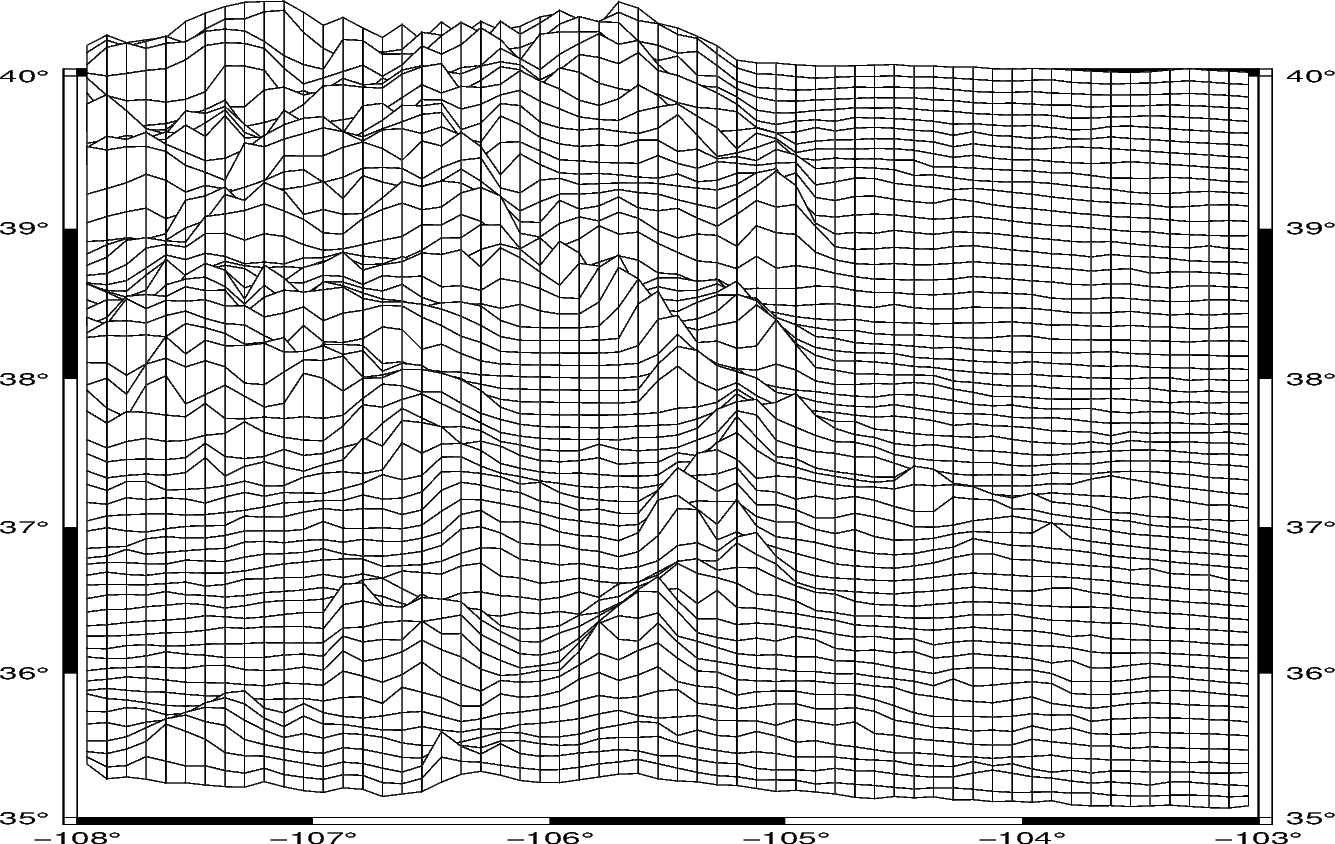
The pygmt.Figure.grdview method takes the grid input. The perspective argument changes the azimuth and angle of the viewpoint; the default is [180, 90], which is looking directly down on the figure and north is “up”. The zsize argument sets how tall the three-dimensional portion appears.

The default figure surface is mesh plot.

fig = pygmt.Figure()
fig.grdview(
    grid=grid,
    # Sets the view azimuth as 180 degrees, and the view angle as 30 degrees
    perspective=[180, 30],
    # Sets the x- and y-axis labels, and annotates the west, south, and east axes
    frame=["xa", "ya", "WSnE"],
    # Sets a Mercator projection on a 15-centimeter figure
    projection="M15c",
    # Sets the height of the three-dimensional relief at 1.5 centimeters
    zsize="1.5c",
)
fig.show()

Out:

<IPython.core.display.Image object>

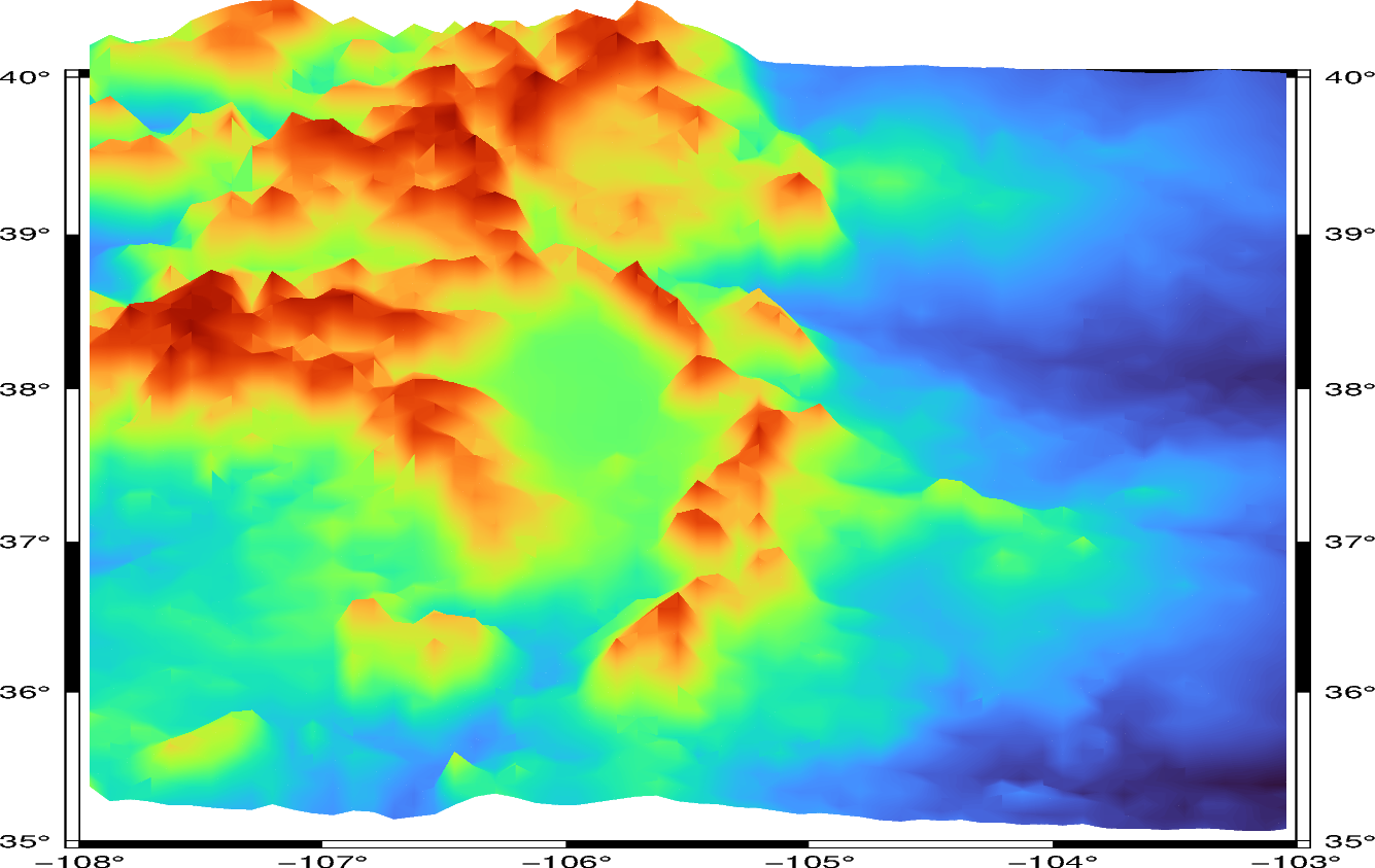
The figure surface type can be set with the surftype parameter. The default CPT is turbo.

fig = pygmt.Figure()
fig.grdview(
    grid=grid,
    perspective=[180, 30],
    frame=["xa", "ya", "WSnE"],
    projection="M15c",
    zsize="1.5c",
    # Sets the surface type to solid
    surftype="s",
)
fig.show()

Out:

<IPython.core.display.Image object>

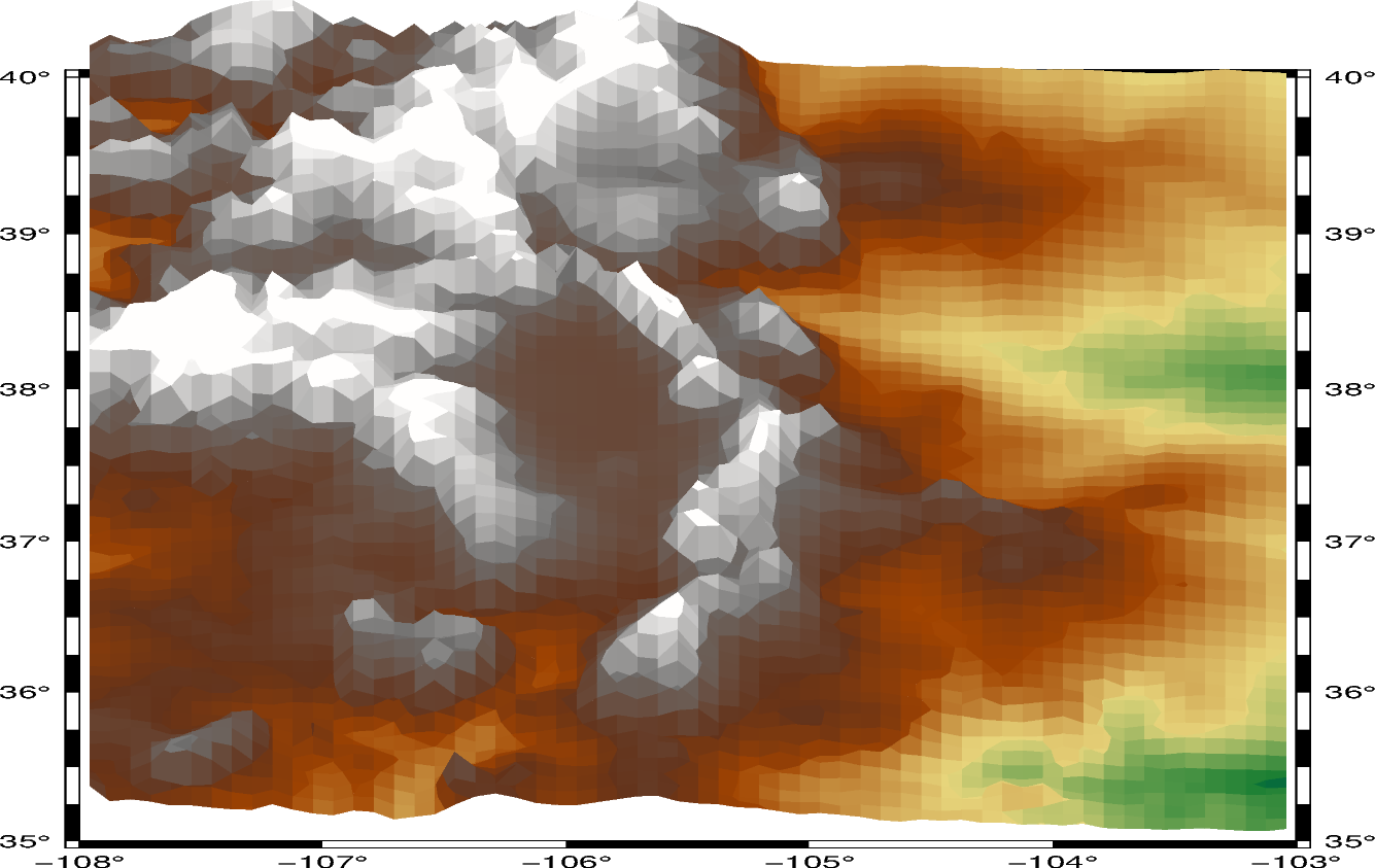
The CPT can be set with the cmap parameter.

fig = pygmt.Figure()
fig.grdview(
    grid=grid,
    perspective=[180, 30],
    frame=["xa", "yaf", "WSnE"],
    projection="M15c",
    zsize="1.5c",
    surftype="s",
    # Set the CPT to "geo"
    cmap="geo",
)
fig.show()

Out:

<IPython.core.display.Image object>

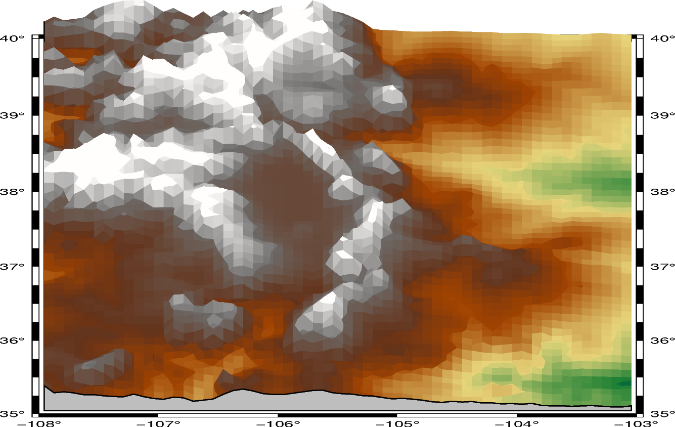
The plane argument sets the elevation and color of a plane that provides a fill below the surface relief.

fig = pygmt.Figure()
fig.grdview(
    grid=grid,
    perspective=[180, 30],
    frame=["xa", "yaf", "WSnE"],
    projection="M15c",
    zsize="1.5c",
    surftype="s",
    cmap="geo",
    plane="1000+ggrey",
)
fig.show()

Out:

<IPython.core.display.Image object>

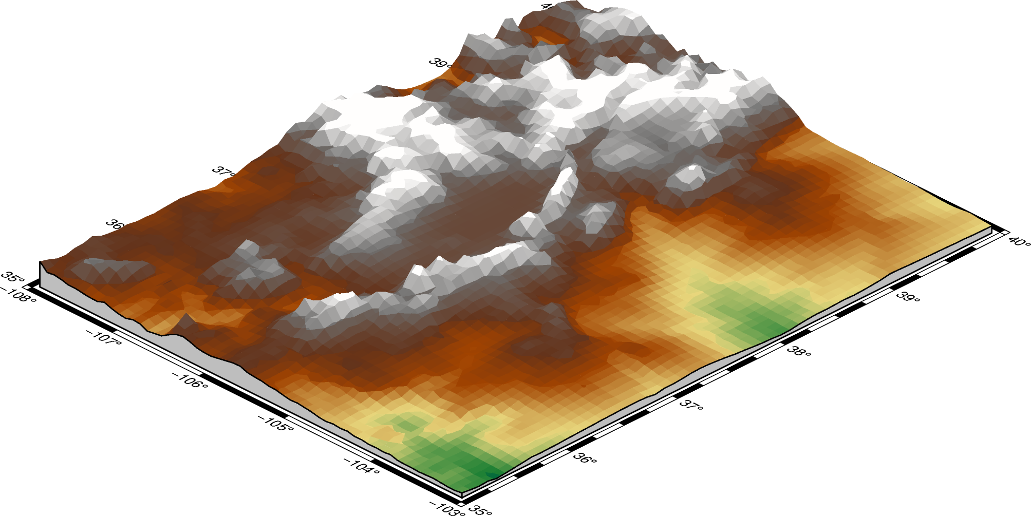
The perspective azimuth can be changed to set the direction that is “up” in the figure.

fig = pygmt.Figure()
fig.grdview(
    grid=grid,
    # Set the azimuth to 135 degrees and the elevation to 30 degrees
    perspective=[135, 30],
    frame=["xa", "yaf", "WSnE"],
    projection="M15c",
    zsize="1.5c",
    surftype="s",
    cmap="geo",
    # Set the elevation of the plane at 1,000 meters and the color to grey
    plane="1000+ggrey",
)
fig.show()

Out:

<IPython.core.display.Image object>

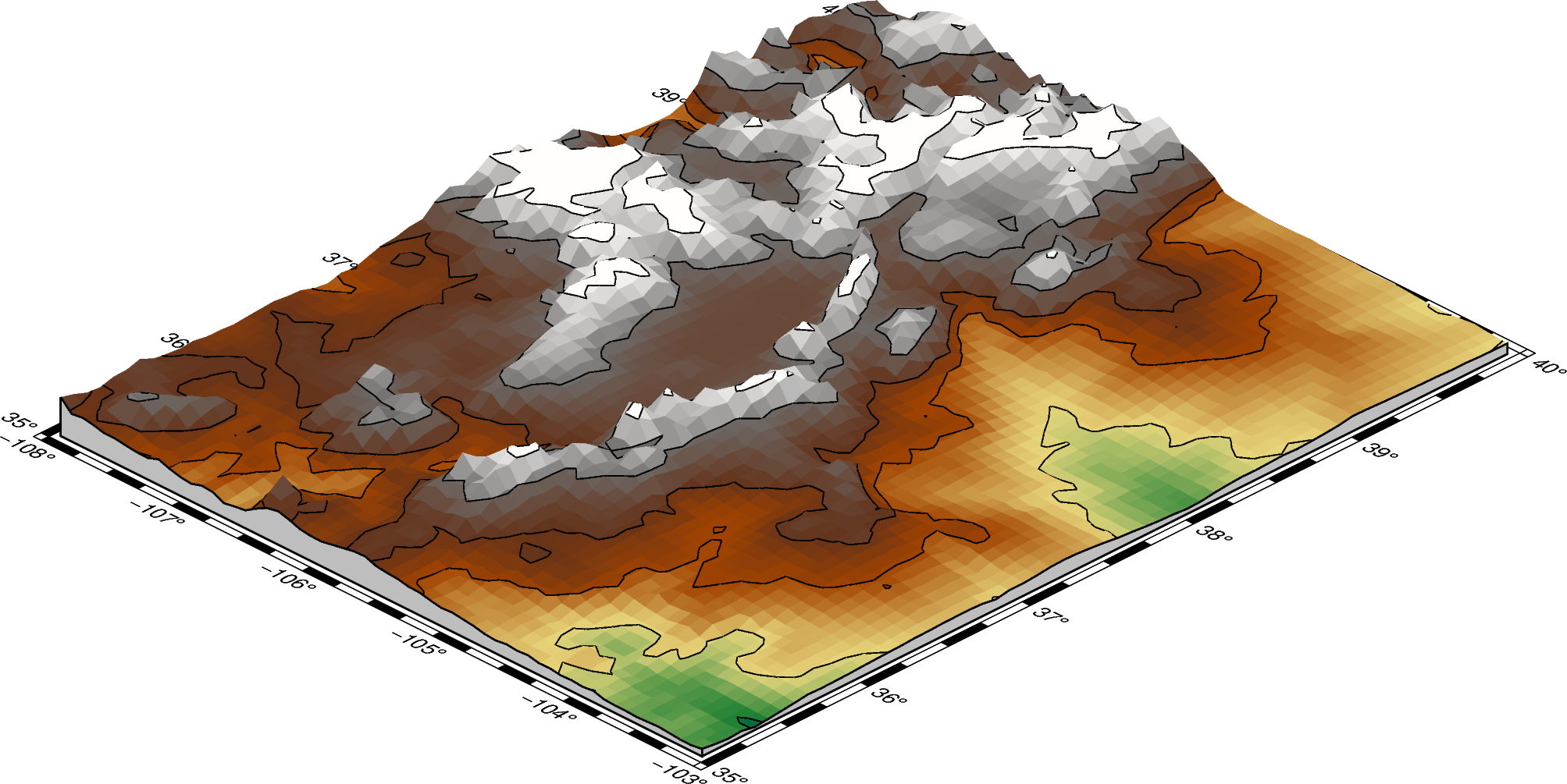
The contourpen parameter sets the pen used to draw contour lines on the surface.

fig = pygmt.Figure()
fig.grdview(
    grid=grid,
    perspective=[135, 30],
    frame=["xaf", "yaf", "WSnE"],
    projection="M15c",
    zsize="1.5c",
    surftype="s",
    cmap="geo",
    plane="1000+ggrey",
    # Set the contour pen thickness to "0.5p"
    contourpen="0.5p",
)
fig.show()

Out:

<IPython.core.display.Image object>

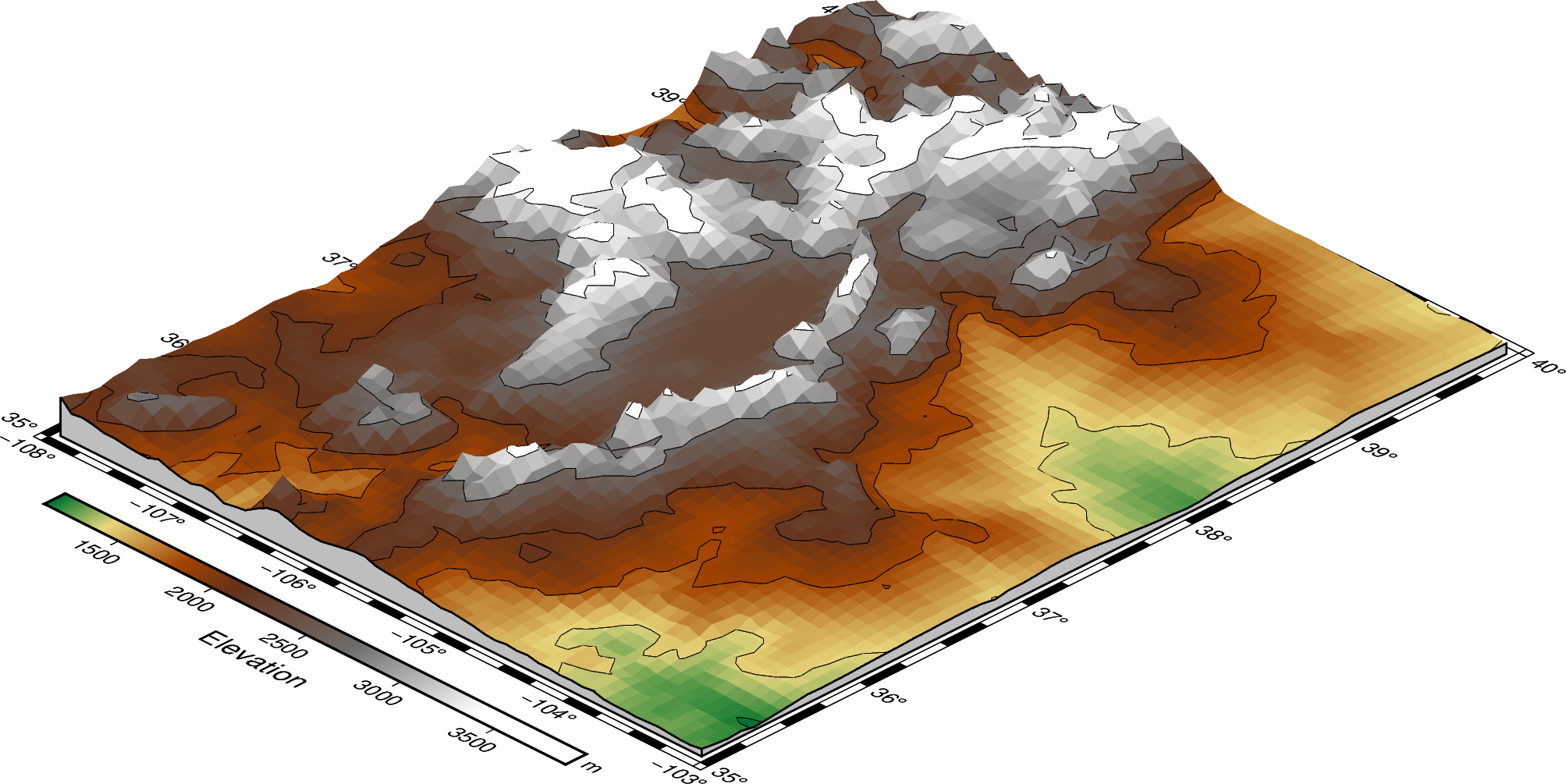
pygmt.Figure.colorbar can be used to add a color bar to the figure. The cmap argument does not need to be passed again. To keep the color bar’s alignment similar to the figure, it also takes a perspective argument.

fig = pygmt.Figure()
perspective = [135, 30]
fig.grdview(
    grid=grid,
    perspective=perspective,
    frame=["xaf", "yaf", "WSnE"],
    projection="M15c",
    zsize="1.5c",
    surftype="s",
    cmap="geo",
    plane="1000+ggrey",
    contourpen="0.1p",
)
fig.colorbar(perspective=perspective, frame=["a500", "x+lElevation", "y+lm"])
fig.show()

Out:

<IPython.core.display.Image object>